
Advanced Propagation Techniques for Long-Distance Ham Radio Operations

As we navigate the evolving landscape of amateur radio from my vantage on Caswell Beach and Oak Island in North Carolina—where the Atlantic’s horizon often serves as a natural boundary for line-of-sight communications—understanding propagation becomes essential for extending our reach beyond the immediate coastal confines. Consider the events following Hurricane Maria in 2017, when Puerto Rican hams relied on HF propagation to connect with the mainland. As documented in ARRL reports from that October, operators on frequencies like 7.268 MHz LSB exploited favorable ionospheric conditions to relay over 5,000 messages to the National Hurricane Center, bypassing devastated infrastructure and facilitating aid distribution. Such successes hinge on predicting how radio waves interact with the atmosphere, influenced by solar activity that can either enhance or disrupt signals. In your region, where storms frequently challenge VHF/UHF reliability, mastering high-frequency (HF) propagation—spanning 3 to 30 MHz—enables consistent long-distance links, from statewide nets to transcontinental contacts.
This exploration delves deeply into HF propagation mechanics, the ongoing solar cycle’s implications, and analytical tools like VOACAP for forecasting viable paths. Aimed at bridging the gap for Technician-class operators venturing into General privileges and providing refinement for Extra-class veterans, we’ll examine the ionosphere’s role, key solar metrics, modeling methodologies, and practical exercises. As of January 2026, with Solar Cycle 25 having crested its peak around mid-2025 and now entering a gradual decline, conditions remain robust for upper HF bands, though increased geomagnetic disturbances demand vigilant monitoring. The Mechanics of HF Propagation: Ionospheric Interactions and Wave Behavior
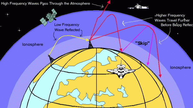
High-frequency radio waves propagate over long distances primarily through skywave, where signals refract off ionized layers in the upper atmosphere rather than following the Earth’s curvature. This refraction occurs in the ionosphere, a region extending from approximately 50 to 600 kilometers altitude, ionized by solar ultraviolet and X-ray radiation. The ionosphere comprises distinct layers: the D layer (50-90 km), E layer (90-150 km), and F layer (150-600 km, splitting into F1 and F2 during daylight). Each layer’s electron density, measured in electrons per cubic centimeter, determines its refractive index for radio waves.
The D layer, densest during daytime, absorbs lower HF frequencies (below 10 MHz) due to collisions between electrons and neutral molecules, limiting daytime range on bands like 80 meters (3.5-4 MHz) to groundwave (surface-hugging paths up to 100 miles). At night, D-layer absorption diminishes, allowing signals to reach higher layers for longer skips. The E layer supports sporadic reflections, useful for 6-meter (50 MHz) “magic band” openings during summer solstices, where signals bounce unpredictably over 1,000 miles. However, the F layer is the workhorse for consistent long-haul: F2, peaking at 300-400 km, enables global paths on 20 meters (14 MHz) via multiple hops, each skip covering 1,000-2,000 miles depending on the maximum usable frequency (MUF).
MUF represents the highest frequency refracted back to Earth at a given angle, calculated as MUF = f_c / sin(θ), where f_c is the critical frequency (proportional to sqrt(electron density)) and θ is the takeoff angle. For low-angle DX (distant contacts), MUF must exceed your operating frequency; otherwise, waves penetrate the ionosphere into space, creating “skip zones” where signals are inaudible (e.g., 200-500 miles on 40 meters daytime). In Caswell Beach, with your proximity to the Atlantic, low takeoff angles (5-15 degrees) favor paths to Europe on 15 meters (21 MHz) during high solar activity, but require antennas like beams or verticals to achieve them.
Solar flares and coronal mass ejections (CMEs) introduce variability: X-class flares can black out HF by enhancing D-layer absorption, as seen in the January 19, 2026, S4 solar radiation storm reported by NOAA, which disrupted polar routes but spared mid-latitudes NOAA S4 Storm January 19, 2026. Geomagnetic storms, rated by K-index (0-9), distort the F layer, potentially opening auroral paths on 10 meters (28 MHz) but closing equatorial routes.
To visualize the ionosphere’s structure:
https://www.swpc.noaa.gov/phenomena/ionosphere

Regions of the ionosphere, showing the D, E, and F layers, UCAR/Randy Russell
Characteristics of different ionospheric layers
Solar Energy Utilization → Term
(Diagram illustrating the ionospheric layers (D, E, F1, F2) and their impact on radio wave refraction; source: antenna-theory.com antenna-theory.com
Solar Cycles and Their Impact on Propagation
Solar cycles, lasting approximately 11 years, drive ionospheric ionization through sunspot activity. Sunspots, dark magnetic regions on the photosphere, correlate with increased UV output, boosting electron density and thus MUF. The smoothed sunspot number (SSN) quantifies this: Cycle 25, which began in December 2019, reached a peak SSN of around 115 in mid-2025, per NOAA’s Solar Cycle Progression data, before declining to about 91.8 in November 2025 and rebounding slightly to 124 in December NOAA Solar Cycle Progression. As of January 2026, with SSN hovering near 100-120, we’re in the post-peak phase, still favoring higher bands (10-15 meters) for daytime DX, but with increasing absorption on lower bands due to lingering high solar flux.
Key indices for daily forecasting include:
Solar Flux Index (SFI): Measured at 10.7 cm wavelength (2.8 GHz), SFI tracks coronal activity. Values above 150 (common in 2025-2026) elevate MUF, enabling 10-meter openings to Asia from NC during mornings. Current SFI as of January 2026 hovers around 180-200, based on recent NOAA readings, supporting robust propagation but risking blackouts from flares NOAA Solar Flux Chart.
K and A Indices: Planetary (Kp) and equivalent amplitude (Ap) measure geomagnetic field disturbances. Kp >5 indicates storms that can enhance auroral VHF but degrade HF equatorial paths. The January 19, 2026, G4 geomagnetic storm (Kp=8) disrupted mid-HF but opened polar routes NOAA G4 Storm January 19, 2026.
Sunspot Number (SSN): Daily values fluctuate; Cycle 25’s decline projects SSN dropping to 50-70 by late 2026, shifting optimal bands downward to 20-40 meters, per NOAA predictions NOAA Sunspot Graph.
For your Caswell Beach station, high SFI means reliable 15-meter paths to Europe (e.g., 21.200 MHz USB) from 1200-1800 UTC, but monitor for CME-induced blackouts, which can last hours to days.
Here’s a recent solar flux chart from NOAA illustrating Cycle 25’s trajectory:

https://www.wm7d.net/hamradio/solar/
Solar Integration → Term
(NOAA Space Weather Prediction Center solar flux chart for Cycle 25, showing observed (blue) vs. predicted (magenta) values up to January 2026; source: swpc.noaa.gov swpc.noaa.gov
And a sunspot number graph for context:
(Graph of Solar Cycle 25 sunspot numbers, highlighting the 2025 peak and early 2026 decline; source: swpc.noaa.gov swpc.noaa.gov
Propagation Modeling Tools: VOACAP and Beyond
To predict rather than guess, tools like VOACAP (Voice of America Coverage Analysis Program) simulate paths based on inputs such as location, time, power, antennas, and solar indices. Developed by the U.S. Department of Commerce, VOACAP uses ionospheric models (e.g., IRI-2016) to compute reliability, signal-to-noise ratio (SNR), and MUF for point-to-point links. Free downloads are available from voacap.com, with online versions for quick runs VOACAP Online.
Using VOACAP: Input transmitter/receiver coordinates (e.g., your 33.9°N, 78.1°W in Caswell Beach to a contact at 40.7°N, 74.0°W in New York), select mode (SSB), power (100W), antennas (dipole at 10m height), and current indices (SFI=180, SSN=110, K=3). It outputs hourly reliability percentages, recommending bands like 20m for 80% success daytime in January 2026.
For deeper analysis, adjust for noise floors (urban vs. rural) or seasonal variations—winter favors lower bands due to longer nights. Alternatives include HamCAP (free at dxatlas.com) for quick maps HamCAP Download and PropView (part of DXLab suite, dxlabsoftware.com) for beacon monitoring PropView.
Here’s a screenshot of VOACAP’s interface during a sample run:
(Screenshot of VOACAP propagation prediction software, displaying input parameters and output reliability chart for an HF path; source: voacap.com voacap.com
And an MUF map from NOAA for global visualization:
(HF propagation MUF map from NOAA, showing maximum usable frequencies across regions for current conditions; source: swpc.noaa.gov swpc.noaa.gov
Interactive Propagation Exercises: Hands-On Forecasting
To upskill, engage in exercises that apply these concepts. First, monitor beacons: Use the International Beacon Project (IARU) on frequencies like 14.100 MHz, where stations transmit sequentially from 18 locations worldwide. From Caswell Beach, tune to 20m at dawn (1100 UTC) and log heard beacons—strong signals from Europe indicate open paths, correlating with SFI >150. Software like Faros (dxatlas.com/faros) automates this, plotting propagation in real-time Faros Software.
Exercise 1: Basic MUF Calculation. Estimate MUF for a 1,000-mile path: If critical frequency f_c = 8 MHz (from NOAA real-time data at prop.kc2g.com) KC2G Propagation, and takeoff angle θ = 20 degrees (from a 30m-high dipole), MUF ≈ 8 / sin(20°) ≈ 23.4 MHz. Thus, 15m (21 MHz) should work, but 10m (28 MHz) may not.
Exercise 2: VOACAP Path Prediction. Download VOACAP and input your location to Miami (25.8°N, 80.2°W), 100W, January 2026 1800 UTC, SFI=180. Expect 90% reliability on 20m, dropping to 60% on 10m due to declining cycle. Vary SSN (e.g., 50 for 2027 projection) to see band shifts.
Exercise 3: Geomagnetic Impact Simulation. Using NOAA’s real-time K-index (e.g., K=4 on January 20, 2026), rerun VOACAP—higher K reduces reliability by 20-30% on polar paths but may enhance equatorial.
These exercises, repeatable weekly, build intuition. Track via logs or apps like HamAlert (hamalert.org) for band opening notifications HamAlert.
Current Solar Cycle Predictions and Strategies for 2026
Solar Cycle 25, as tracked by NOAA, peaked at SSN ~115 in 2025 and is now declining, with monthly values dipping to 91.8 in November 2025 before a slight uptick to 124 in December NOAA Cycle 25 Update. By mid-2026, expect SSN 70-90, shifting prime bands from 10-15m to 17-30m for daytime, with 40-80m strengthening at night. This post-maximum phase brings more stable propagation but increased risk from residual flares—e.g., the X-class event on January 18, 2026, captured by NASA’s Solar Dynamics Observatory, which temporarily elevated MUF but caused D-layer blackouts NASA Flare January 18, 2026.
For Caswell Beach strategies: Favor 20m (14.200-14.350 MHz USB) for East Coast nets during mornings, transitioning to 40m (7.200-7.300 MHz LSB) evenings. Monitor NOAA’s Space Weather Prediction Center for 3-day forecasts of SFI/K-index, adjusting antennas (e.g., lower dipoles for NVIS on disturbed days). With minimum projected around 2030-2031, plan for gradual reliance on lower bands, but 2026’s lingering activity supports experimental modes like FT8 on 10m for sporadic E-layer openings.
Here’s a sunspot progression graph for Cycle 25:
(Solar cycle sunspot number graph for Cycle 25, showing observed data through January 2026 with predicted decline; source: swpc.noaa.gov swpc.noaa.gov
Advanced Tuning and Mitigation Techniques
For pros, refine models with antenna patterns: VOACAP accepts NEC files for gain/directivity, optimizing for your beachside vertical (high ground conductivity enhances low-angle radiation). Mitigate absorption with mode selection—SSB for voice, but digital like JS8Call (js8call.com) for weak signals during high K-index JS8Call. Use real-time ionograms from digisondes (e.g., Lowell Digisonde at umlcar.uml.edu) to verify f_c Lowell Digisonde.
In NC, leverage local resources like the NC ARRL Section for propagation reports during drills NC ARRL. Forward-looking: As Cycle 26 approaches (onset 2029-2032), tools like SolarHam (solarham.net) provide ensemble forecasts SolarHam.
FAQs: Addressing Propagation Queries
How does solar maximum affect NC ops? Higher MUF opens 10m, but more blackouts; monitor daily.
Best tool for beginners? Start with online VOACAP—no install needed.
Predicting skips? Use MUF maps; avoid grayline for NVIS.
Cycle 25 endgame? By 2027, focus 30-80m; prepare now.
Action Plan: Master Propagation Today
Download VOACAP; run a path from Caswell Beach to Europe.
Monitor beacons daily; log vs. indices.
Join a prop net like the Propagation Net on 14.233 MHz.
Exercise: Forecast your next DX, validate post-contact.
Track Cycle 25 via NOAA alerts.
Next: Maintenance.
For NC, visit ncarrl.org ncarrl.org.
As always, if you find bad links, let me know at n0njy.qsl.net. If you find mistakes, let me know. I don’t make money from this blog, I don’t get paid, by anyone. I pass this information on freely. I do ask if you take some of my work to share, that you retain my name and call sign (N0NJY) on the work, since it is my work and no one else’s. Thanks. 73
Need to save this for future reference. Just getting into the hf world